https://sgugger.github.io/the-1cycle-policy.html
Here, we will dig into the first part of Leslie Smith's work about setting hyper-parameters (namely learning rate, momentum and weight decay). In particular, his 1cycle policy gives very fast results to train complex models. As an example, we'll see how it allows us to train a resnet-56 on cifar10 to the same or a better precision than the authors in their original paper but with far less iterations.
By training with high learning rates we can reach a model that gets 93% accuracy in 70 epochs which is less than 7k iterations (as opposed to the 64k iterations which made roughly 360 epochs in the original paper).
This notebook contains all the experiments. They are done with the same data-augmentation as in this original paper with one minor tweak: we random flip the picture horizontally and a random crop after adding a padding of 4 pixels on each side. The minor tweak is that we don't color the padded pixels in black, but use a reflection padding, since it's the one implemented in the fastai library. This is probably why we get slightly better results than Leslie when doing the experiments with the same hyper-parameters.
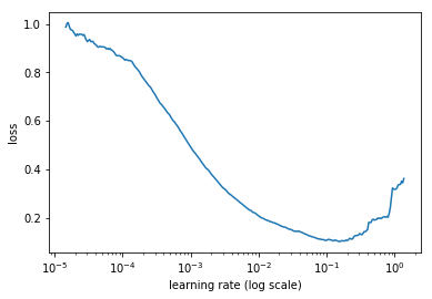
We have already seen how to implement the learning rate finder. Begin to train the model while increasing the learning rate from a very low to a very large one, stop when the loss starts to really get out of control. Plot the losses against the learning rates and pick a value a bit before the minimum, where the loss still improves. Here for instance, anything between 10−2 and 3×10⁻² seems like a good idea.
This was already an idea of the same author and he completes it in his last article with a good approach to adopt during training.
He recommends to do a cycle with two steps of equal lengths, one going from a lower learning rate to a higher one than go back to the minimum. The maximum should be the value picked with the Learning Rate Finder, and the lower one can be ten times lower. Then, the length of this cycle should be slightly less than the total number of epochs, and, in the last part of training, we should allow the learning rate to decrease more than the minimum, by several orders of magnitude.
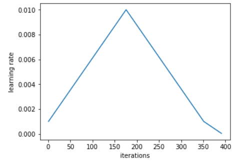
The idea of starting slower isn't new: using a lower value to warm-up the training is often done, and this is exactly what the first part is achieving. Leslie doesn't recommend to switch to a higher value directly, however, but to rather slowly go there linearly, and to take as much time going up as going down.
What he observed during his experiments is that the during the middle of the cycle, the high learning rates will act as regularization method, and keep the network from overfitting. They will prevent the model to land in a steep area of the loss function, preferring to find a minimum that is flatter. He explained in this other paper how he observed that by using this policy, approximates of the hessian were lower, indicating that the SGD was finding a wider flat area.
Then the last part of the training, with descending learning rates up until annihilation will allow us to go inside a steeper local minimum inside that smoother part. During the par with high learning rates, we don't see substantial improvements in the loss or the accuracy, and the validation loss sometimes spikes very high, but we see all the benefits of doing this when we finally lower the learning rates at the end.
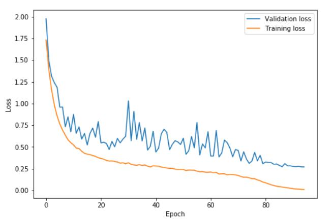
In this graph, the learning rate was rising from 0.08 to 0.8 between epochs 0 and 41, getting back to 0.08 between epochs 41 and 82 then going to one hundredth of 0.08 in the last few epochs. We can see how the validation loss gets a little bit more volatile during the high learning rate part of the cycle (epochs 20 to 60 mostly) but the important part is that on average, the distance between the training loss and the validation loss doesn't increase. We only really start to overfit at the end of the cycle, when the learning rate gets annihilated.
Surprisingly, applying this policy even allows us to pick larger maximum learning rates, closer to the minimum of the plot we draw when using the learning rate finder. Those trainings are a bit more dangerous in the sense that the loss can go too far away and make the whole thing diverge. In those cases, it can be worth to try with a longer cycle before going to a slower learning rate, since a long warm-up seems to help.
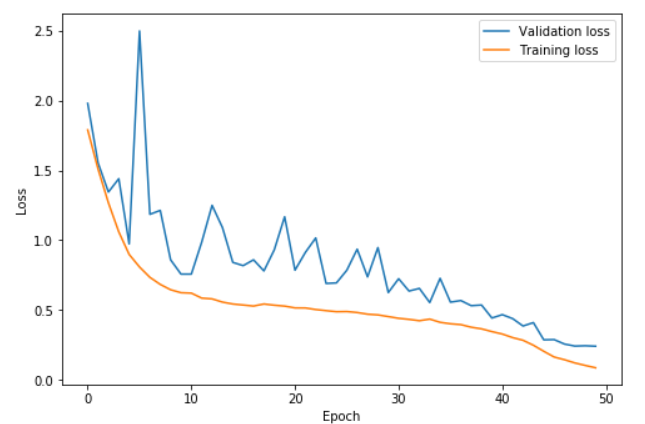
In this graph, the learning rate was rising from 0.15 to 3 between epochs 0 and 22.5, getting back to 0.15 between epochs 22.5 and 45 then going to one hundredth of 0.15 in the last few epochs. With very high learning rates, we get to learn faster and prevent overfitting. The difference between the validation loss and the training loss stays extremely low up until we annihilate the learning rates. This is the phenomenon Leslie Smith describes as super convergence.
With this technique, we can train a resnet-56 to have 92.3% accuracy on cifar10 in barely 50 epochs. Going to a cycle of 70 epochs gets us at 93% accuracy.